Visualizing the Perceptron Learning Algorithm
Introduction
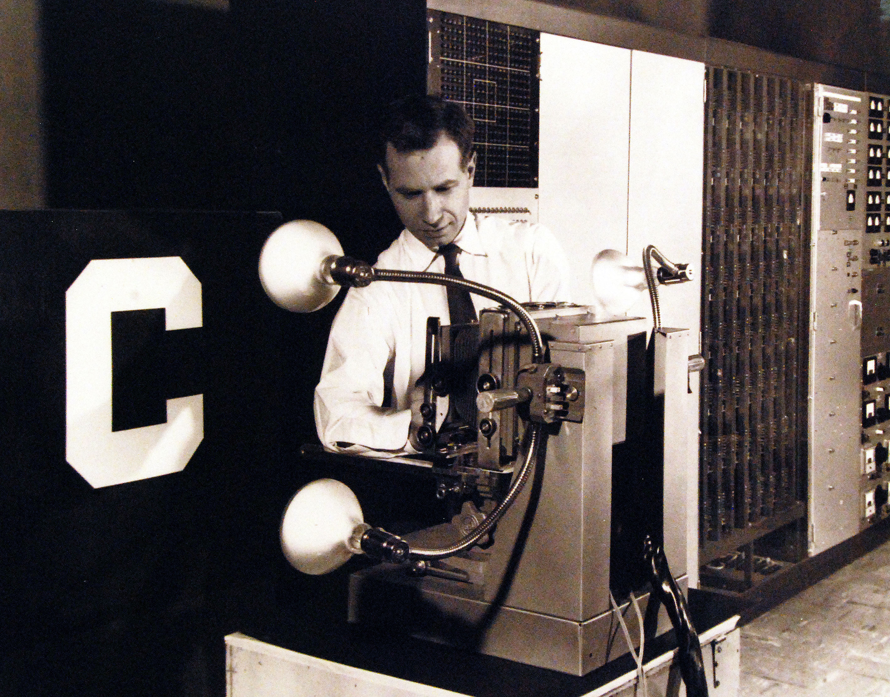
The perceptron is an early innovation made in the field of machine learning. Designed to mimic the neurons in the human brain, it went on to build the foundations of today’s neural networks. The perceptron was developed by Frank Rosenblatt at the Cornell Aeronautical Laboratory (source).
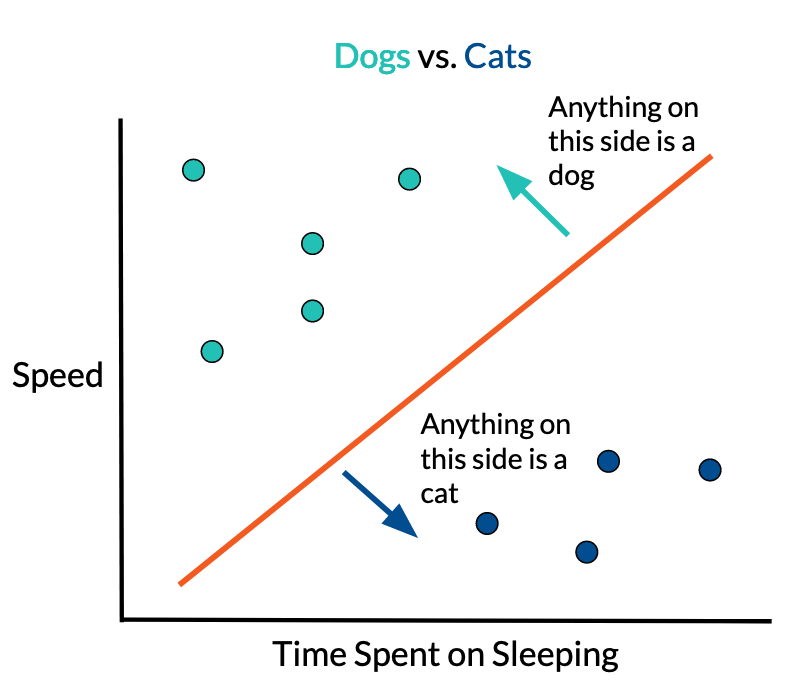
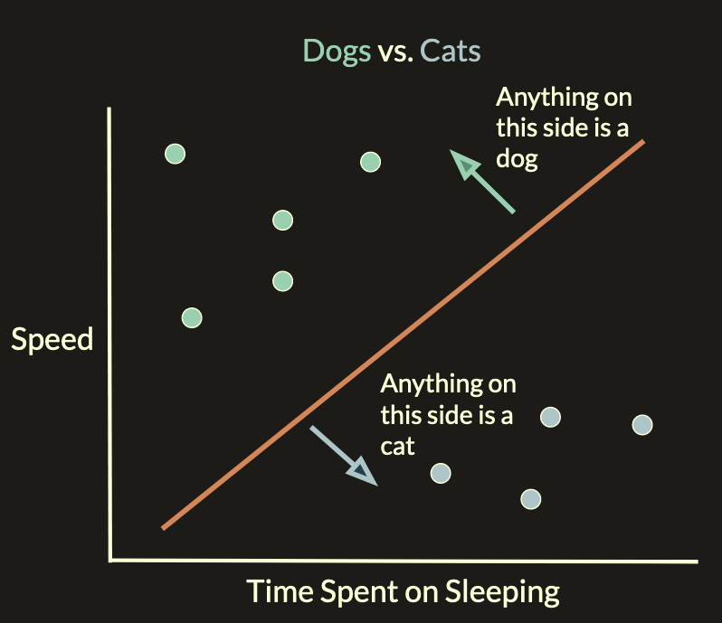
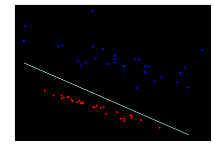
To truly understand how the perceptron works, we must first view it from a geometrical perspective before getting into the “neural” aspect of it. A single perceptron is a linear classifier – it separates two groups using a line. Given a training dataset, the perceptron learns by readjusting itself based on points it misclassified (points on the wrong side of the line) at every timestep.
When the problem is in 2D, it becomes very easy for us humans to figure out a solution to the problem – we can simply eyeball a line that separates two groups. But when it comes to higher dimensions (or simply just programming a computer to do this process for us), we will need a more well-defined algorithm.
The Perceptron Learning Algorithm
Distance from a point to the line
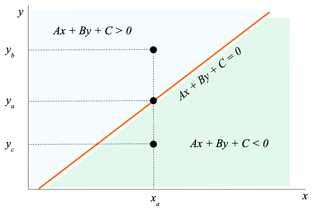
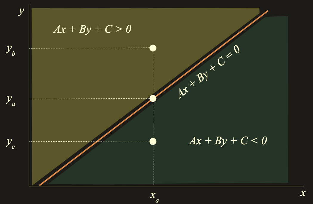
To write an algorithm that finds a line that separates the two groups, we must first find a way to figure out whether a given point is above or below the line. The formula for the distance (sign included) between a point $(x_a, y_a)$ and a line $Ax + By + C = 0$ is
\[d = \frac{Ax_a + By_a + C}{\sqrt{A^2 + B^2}}.\]Since we are mainly focused on the sign of the result (whether the point is above or below) and since $\sqrt{A^2 + B^2} \geq 0$ by definition of square root, just knowing whether
\[Ax_a + By_a + C > 0\]will let us know if the point $(x_a, y_a)$ is above the line.
Find multiple proofs of this formula here
Another way to look at it
Intuitively, we know that the equation of the line is $Ax + By + C = 0$. That means that if the point $(x_a, y_a)$ were on the line, then $Ax_a + By_a + C = 0$. If the point $(x_a, y_b)$ is above the line, we know that $y_b > y_a$ and since the $x$-values are the same for both points, we know that $Ax_a + By_b + C > 0$. Similarly, we can see how a point $(x_a, y_c)$ under the line would have $Ax_a + By_b + C < 0$.
Note: This is assuming that the coefficients are positive. If not, the top region could perhaps be where $Ax + By + C < 0$ instead and the bottom be $Ax + By + C > 0$. You will see this as you interact with a model later in the post.
Using the formula for finding misclassified points
In summary, we can make a prediction for a point $(x_a, y_a)$ by computing
\[\text{sgn}(Ax_a + By_b + C),\]where the value of $1$ denotes the point is part of one group and a value of $-1$ denotes the point is part of the other.
The $\text{sgn}$ function computes the sign of the input. It is defined as follows:
\[\text{sgn}(x) = \begin{cases} 1 & \text{if } x > 0 \\ 0 & \text{if } x = 0 \\ -1 & \text{if } x < 0 \end{cases}\]
Given a training dataset – set of points $(x, y, a)$ were $x$ and $y$ are coordinates and $a$ is $1$ or $-1$ depending on which group the point is part of – we can find misclassified points by finding points whose $a$ value is different from the prediction.
The “learning” in perceptron learning
Here is the outline of the perceptron learning algorithm:
This algorithm will update the line $Ax + By + C = 0$ to have new coefficients that ideally separate the two groups in the data.
The natural question is why these updates ($A \leftarrow A + a \cdot x \dots$) work. There are multiple ways to explain but we will offer the most intuitive explanation. Suppose we have a datapoint $(x_a, y_a, 1)$ which is misclassified. This means that
\[\text{sgn}(Ax_a + By_a + C) = -1\] \[\implies Ax_a + By_a + C < 0.\]We want to change the line such that $Ax_a + By_a + C > 0$. If we increase $A$, $B$, and $C$ we know that the value $Ax_a + By_a + C$ will increase, thereby getting closer to positive territory (assuming $x_a$ and $y_a$ are positive). If one of the terms – suppose $x_a$ was negative – we would want to decrease $A$. We can simply add $x_a$ to $A$ to achieve these results.
When a datapoint $(x_a, y_a, -1)$ is misclassified, our model predicted
\[\text{sgn}(Ax_a + By_a + C) = 1\] \[\implies Ax_a + By_a + C > 0.\]We simply must perform the same updates to the coefficients but in the reverse direction – and for that reason we update each weight by the product of $a$ and the respective variable $x$ or $y$.
This is by no means a proof. Other intuitive explanations of why these updates work can be found here and here.
Below is a Desmos embedding that demonstrates how weights can get updated. The top row in the left sidebar gives the current raw prediction (no sign function) of the perceptron $Ax + By + C$. Increase or decrease the coefficients $A, B,$ and $C$ by moving the sliders underneath. Suppose the point $(7,9)$ was misclassified. That means that the point should be on the other side of the line (notice the orange and blue sides of the line below). In this case when the coefficients increase, the line moves so that eventually the point is on the other side of the line. If you make the point with negative values, the direction in which the various coefficients will have to change will be different (and be according to the algorithm stated earlier).
Learning Rate
The learning rate, “$r$”, scales how much we correct our perceptron for each misclassified point. High learning rate means we might overcorrect, meaning the line will bounce around the data more. Low learning rate means that we might undercorrect, meaning the line will not move much and hence will take a longer time to train. See the algorithm below to view how this constant is factored into weight updates:
Try it Yourself!
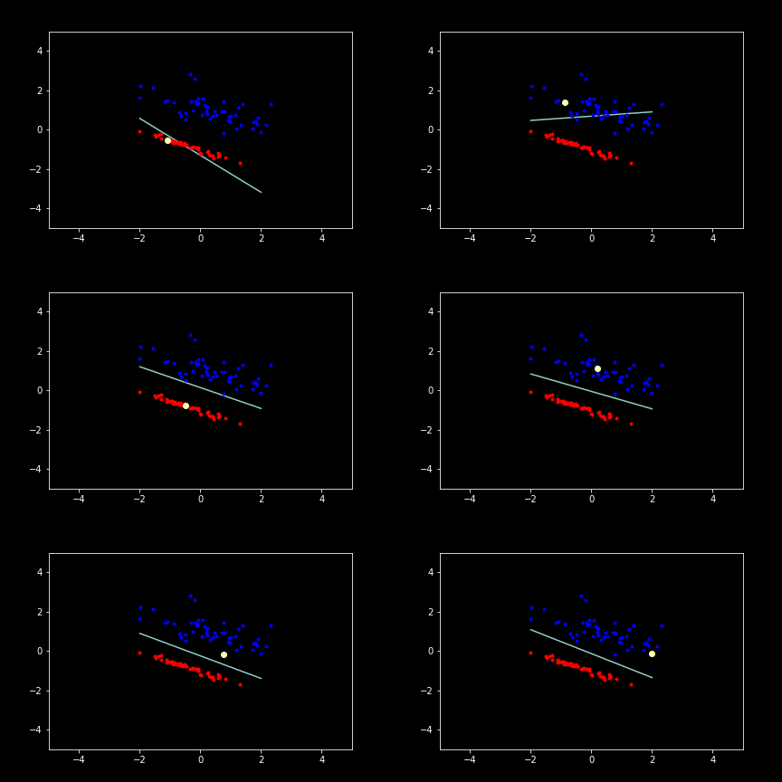
Click on different locations on the graph to generate datapoints. Click on the “Switch Color” button to change which group the next generated points are part of. Finally, click the “Train Perceptron” button to start the training.
The yellow highlighted point during training represents the current point from which the coefficients of the line are being updated by. Click “Reset” or reload the page to reset to get a new initial plane.
“Neuron” Representation of the Perceptron
$n$-dimensions and vectors
Visualizing 3D space
We can also apply the perceptron learning algorithm to 3D data. In this case we have a plane
\[Ax + By + Cz + D = 0,\]where on one side $Ax + By + Cz + D > 0$ and on the other $Ax + By + Cz + D < 0$.
Click and drag the mouse around to view the data from different angles and scroll to zoom. Click on the “Train Perceptron” button to view the animation. Click “Reset” or reload the page to reset to get a new initial plane.
Vectors for beyond 3D
So far all of the calculations have been done on 2-D space – each point has two coordinates $x$ and $y$ (in 3D space we add a $z$ coordinate to it). But if we switch out the notation from
\[A \leftarrow A + a \cdot x \\ B \leftarrow B + a \cdot y \\ C \leftarrow C + a \cdot 1 \\\]to
\[w_0 \leftarrow w_0 + a \cdot 1 \\ w_1 \leftarrow w_1 + a \cdot x_1 \\ w_2 \leftarrow w_2 + a \cdot x_2 \\\]$A$ became $w_1$, $B$ became $w_2$, and $C$ became $w_0$.
$x$ became $x_1$ and $y$ became $x_2$.
we can then see a clear pattern. Expressed as vectors, we can instead write these updates as
\[\vec{w} \leftarrow \vec{w} + a \cdot \vec{x}.\]This vector can extend to any dimensions needed, meaning that our perceptron can have as many inputs as needed.
Anatomy of a Perceptron
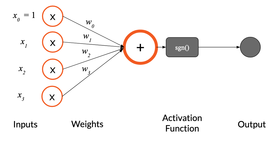
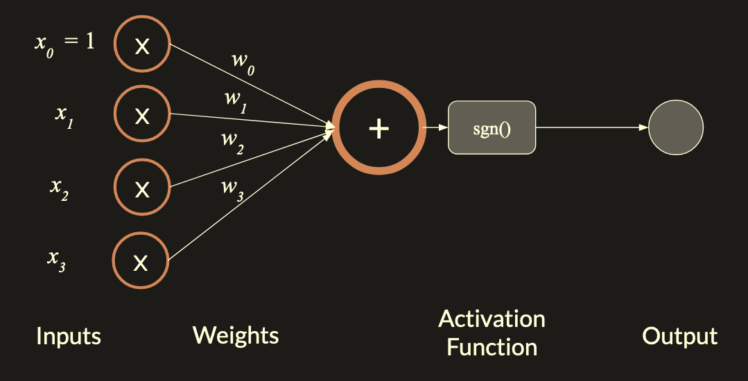
Since it becomes difficult to graph $n$-dimensional data, a better way to graphically represent the perceptron is as a “neuron” which gets $n$ inputs. Each of these inputs is multiplied by the respective weight $w_n$ and all of the products are summed up. The sum is then put through an activation function, in this case the $\text{sgn}$ function.
Non-linearly separable data
One caveat with the perceptron learning algorithm is that it cannot separate any kind of arbitrary data. Specifically, the algorithm requires that the data is linearly separable, meaning that there exists a line that separates the data into the two groups (i.e. there does indeed exist a linear solution). If the data is not linearly separable, the line will end up bouncing around, never halting. Run the example below to see how that happens.
Find a proof that the algorithm converges on linearly separable data here.
Extending from Perceptrons
Other activation functions
You can use activation functions other than the $\text{sgn}$ function. Check out the examples below:
These different activation functions can allow prediction to not just be a discrete value (e.g. $1$ or $-1$) but rather be a specifically scaled, continuous set of numbers that could be the output.
Neural networks
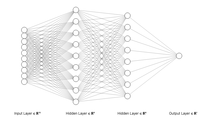
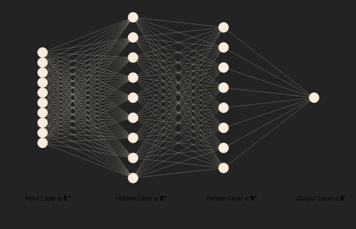
Multi-layered perceptrons are sets of perceptrons linked together to form more complex models. These perceptrons have non-linear activation functions, allowing the model to be able to handle data that are not linearly separable.
These multi-layered perceptrons became now what are called feed-forward artificial neural networks, from which a plethora of other kinds of neural networks were built from later on. The beauty of this is that the powerful properties of these neural networks all stem from a swarm of perceptrons that interact with each other.
Note: there are kinds of neural networks other than feed-forward ones like Hopfield networks
These neurons form the foundation behind the machine learning algorithms of today – Just know that when you use tools like GPT, there are billions of perceptrons hard at work!
Appendix: Algorithm Implementation in Python
Enough with the theory – let’s get into implementing this in code!
Prepare dataset
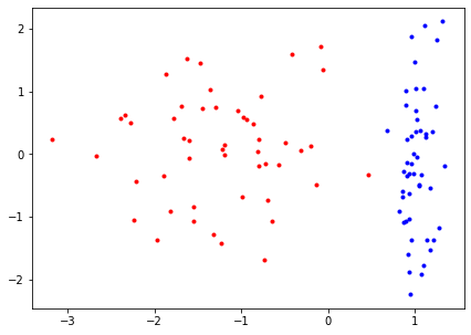
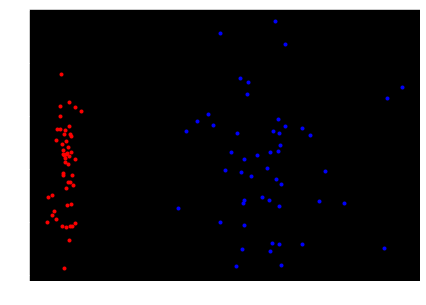
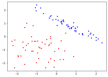
We will create linearly separable data (initially vertical/horizontal) and then rotate it. We want to create linearly separable data because we want the perceptron to converge to a solution (rather than deal with an impossible problem). We want to rotate it to generate interesting data.
1
2
3
from sklearn.datasets import make_classification
import matplotlib.pyplot as plt
plt.style.use('default')
1
2
3
4
5
6
7
8
9
10
11
12
13
14
separable = False
while not separable:
    # create two clusters that are horizontally or vertically next to each other
    samples = make_classification(n_samples=100, n_features=2, n_redundant=0,
                                  n_informative=1, n_clusters_per_class=1, flip_y=-1)

    red = samples[0][samples[1] == 0]
    blue = samples[0][samples[1] == 1]

    # figuring out whether they are linearly separable
    # (either the max y-value of one cluster is less than the min y-value of the other
    # or the max x-value of one cluster is less than the min x-value of the other)
    separable = any([red[:, k].max() < blue[:, k].min() or
                     red[:, k].min() > blue[:, k].max() for k in range(2)])
1
2
3
4
5
# plot the data
plt.figure(figsize=(7, 5))
plt.plot(red[:, 0], red[:, 1], 'r.')
plt.plot(blue[:, 0], blue[:, 1], 'b.')
plt.show()
1
2
3
4
5
6
7
8
9
10
11
12
13
14
15
16
17
18
import numpy as np

# function from https://stackoverflow.com/questions/34372480/rotate-point-about-another-point-in-degrees-python
def rotate(p, origin=(0, 0), degrees=0):
    angle = np.deg2rad(degrees)
    R = np.array([[np.cos(angle), -np.sin(angle)],
                  [np.sin(angle),  np.cos(angle)]])
    o = np.atleast_2d(origin)
    p = np.atleast_2d(p)
    return np.squeeze((R @ (p.T-o.T) + o.T).T)

origin=(np.mean(samples[0], axis=0))

# rotate by a random number of degrees
new_samples_coords = rotate(samples[0],
                            origin=origin, degrees=np.random.randint(30, 80))

samples = (new_samples_coords, samples[1])
1
2
3
4
5
6
7
red = samples[0][samples[1] == 0]
blue = samples[0][samples[1] == 1]

plt.figure(figsize=(7, 5))
plt.plot(red[:, 0], red[:, 1], 'r.')
plt.plot(blue[:, 0], blue[:, 1], 'b.')
plt.show()
We will be splitting the data into training and testing data (a 80-20 split).
1
2
3
4
5
6
7
8
9
10
# we are saving "red" and "blue" variables purely for plotting
red_train = red[20:]
blue_train = blue[20:]

red_test = red[:20]
blue_test = blue[:20]

# these variables are what are used for actual computation
samples_train = (samples[0][20:], samples[1][20:])
samples_test = (samples[0][:20], samples[1][:20])
Train perceptron on the data
The function below returns samples that were misclassified by the line $b + w_1 \cdot x_2 + w_2 \cdot x_2 = 0$
1
2
3
4
5
6
7
8
9
10
11
12
def get_misclassified(samples, w1, w2, b):
    res = []

    for i in range(len(samples[0])):
        x1, x2 = samples[0][i]
        pred = b + w1*x1 + w2*x2
        Y = samples[1][i]

        if (pred > 0) != Y:
            res.append((x1, x2, Y))

    return res
1
LR = 1 # learning rate
1
2
3
4
# Start off with random weights
B = np.random.randint(-10,10)
W_1 = np.random.randint(-10,10)
W_2 = np.random.randint(-10,10)
1
2
3
4
from IPython.display import display, Math

print("Initial weights:")
display(Math(f"{B=}, {W_1=}, {W_2=}"))
Initial weights:
$\displaystyle B=-3, W_1=-5, W_2=8$
1
2
3
4
5
6
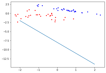
x = np.linspace(-2, 2) # used as the x values to plot our line
plt.figure(figsize=(7, 5))
plt.plot(x, -W_1/W_2 * x - B/W_2) # plot line
plt.plot(red[:, 0], red[:, 1], 'r.') # plot red points
plt.plot(blue[:, 0], blue[:, 1], 'b.') # plot blue points
plt.show()
The code below is what trains our perceptron. Look out for the comments to understand how it works.
1
2
3
4
5
6
7
8
9
10
11
12
13
14
15
16
17
18
19
20
21
22
misclassified = get_misclassified(samples_train, W_1, W_2, B)
while len(misclassified) != 0: # while there are still some misclassified points
    for sample in misclassified:
        # get the sample values
        x1 = sample[0]
        x2 = sample[1]
        y = sample[2]

        # change y so that when we update weights it is in the
        # scale of -1 or 1 rather than 0 or 1
        if y == 0: y = -1

        # update weights
        B = B + y * 1 * LR
        W_1 = W_1 + y * x1 * LR
        W_2 = W_2 + y * x2 * LR

    # calculate the new misclassified points
    misclassified = get_misclassified(samples_train, W_1, W_2, B)

print("Final weights:")
display(Math(f"{B=}, {W_1=}, {W_2=}"))
Final weights:
$\displaystyle B=0, W_1=9.228462336182414, W_2=28.105944178471837$
1
2
3
4
5
6
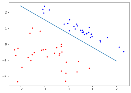
x = np.linspace(-2, 2) # used as the x values to plot our line
plt.figure(figsize=(7, 5))
plt.plot(x, -W_1/W_2 * x - B/W_2) # plot line
plt.plot(red[:, 0], red[:, 1], 'r.') # plot red points
plt.plot(blue[:, 0], blue[:, 1], 'b.') # plot blue points
plt.show()
Test the model
1
2
misclassified = get_misclassified(samples_test, W_1, W_2, B)
len(misclassified)
0
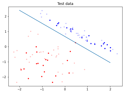
Below is the plot of the line and the testing data. Datapoints that are translucent are training data.
1
2
3
4
5
6
7
8
9
10
11
x = np.linspace(-2, 2) # used as the x values to plot our line
plt.figure(figsize=(7, 5)>>)

plt.plot(red_train[:, 0], red_train[:, 1], 'r.', alpha=0.2) # red train data
plt.plot(blue_train[:, 0], blue_train[:, 1], 'b.', alpha=0.2) # blue train data

plt.plot(red_test[:, 0], red_test[:, 1], 'r.') # red TEST points
plt.plot(blue_test[:, 0], blue_test[:, 1], 'b.') # blue TEST points
plt.plot(x, -W_1/W_2 * x - B/W_2) # plot line
plt.title("Test data")
plt.show()
Making the Animation
1
!mkdir animation # make the folder that will store our results
1
2
3
4
5
6
7
8
9
10
11
12
13
14
15
16
17
18
19
20
21
22
23
24
25
26
27
28
29
30
31
32
33
34
35
36
37
38
39
40
41
42
43
44
45
46
47
48
# Start off with random weights
B = np.random.randint(-10,10)
W1 = np.random.randint(-10,10)
W2 = np.random.randint(-10,10)

count = 0 # used for ordering the intermediate steps that will be also outputed

misclassified = get_misclassified(samples, W1, W2, B)
while len(misclassified) != 0:
    x = np.linspace(-2, 2) # used as the x values to plot our line

    for sample in misclassified:
        plt.close() # delete the old line

        # get the sample values
        x1 = sample[0]
        x2 = sample[1]
        y = sample[2]

        # change y so that when we update weights it is in the scale
        # of -1 or 1 rather than 0 or 1
        if y == 0: y = -1

        # update weights
        B = B + y * 1 * LR
        W1 = W1 + y * x1 * LR
        W2 = W2 + y * x2 * LR

        ax = plt.gca()
        ax.set_xlim([-5, 5])
        ax.set_ylim([-5, 5])

        # plot and save the figure
        plt.title(f'frame number {count}')
        plt.plot(x, -W1/W2 * x - B/W2) # plot line
        plt.plot(red[:, 0], red[:, 1], 'r.') # plot red points
        plt.plot(blue[:, 0], blue[:, 1], 'b.') # plot blue points

        plt.plot(x1, x2, 'o') # point being used to correct the line

        # save the figure, naming it as its index "count"
        plt.savefig(f'./animation/{count}')

        count += 1

    # calculate the new misclassified points
    misclassified = get_misclassified(samples, W1, W2, B)
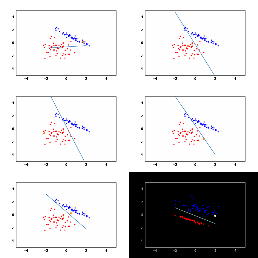
The code below converts the images into a gif
1
2
3
4
5
6
7
8
9
10
11
12
13
14
15
16
17
18
19
20
21
22
23
24
25
26
27
28
29
30
31
32
33
34
35
36
37
38
39
40
41
42
43
44
45
46
47
48
49
50
51
import glob
import contextlib
from PIL import Image

import re

def tryint(s):
    """
    Return an int if possible, or `s` unchanged.
    """
    try:
        return int(s)
    except ValueError:
        return s

def alphanum_key(s):
    """
    Turn a string into a list of string and number chunks.

    >>> alphanum_key("z23a")
    ["z", 23, "a"]

    """
    return [ tryint(c) for c in re.split('([0-9]+)', s) ]

def human_sort(l):
    """
    Sort a list in the way that humans expect.
    """
    l.sort(key=alphanum_key)
    return l

# filepaths
fp_in = "./animation/*.png"
fp_out = "./animation/out.gif"

files = human_sort(glob.glob(fp_in))

# use exit stack to automatically close opened images
with contextlib.ExitStack() as stack:

    # lazily load images
    imgs = (stack.enter_context(Image.open(f))
            for f in files)

    # extract  first image from iterator
    img = next(imgs)

    # https://pillow.readthedocs.io/en/stable/handbook/image-file-formats.html#gif
    img.save(fp=fp_out, format='GIF', append_images=imgs,
             save_all=True, duration=400, loop=0)
Results are in the ‘animations’ folder in the same directory as this notebook. ‘out.gif’ is the animation of the perceptron learning
